Intro to Bayesian methods

This post is really only a test for Rmarkdown integration into Jekyll. Substantively, it is a first lab lesson for applied Bayesian estimation in R.

Load the LearnBayes¹ and Lattice packages.

library(LearnBayes)
library(lattice)

1. Please replicate the sleeping habits analysis using a discrete prior (in the session 1-2)

Setting up a discrete prior

This code is used to create a a discrete prior concerning our beliefs about the proportion college student sleeping habits (p):

p = seq(0.05, 0.95, by = 0.1)
prior = c(1, 5.2, 8, 7.2, 4.6, 2.1, 0.7, 0.1, 0, 0)
prior = prior/sum(prior)

The code above is two-fold, first, it sets up the range of possible proportion values for the amount of students that could be sleeping at least eight hours a night. Second, it creates our discrete prior by specifying our weighted beliefs about each distinct proportion (p).

Next, we plot the our priors for each proportion (p) by using the lot function:

plot(p, prior, type="h", ylab="Prior Probability", xlab="Proportion of College Students with Eight Hours of Sleep")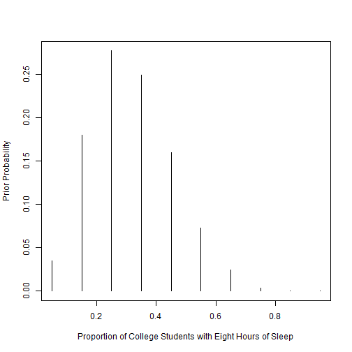

The histogram above visualizes our prior belief in each value of p. The original guess of .3 (from lesson 1-2) being the most probable is highlighted clearly in the histogram. We see that our prior beliefs are greatest between .2 and .4, with.3 being the peak in the middle.

Evidence and Posterior

Next, we want to calculate the posterior probabilities for p by utilizing the data on college student sleeping habits. In the example study, only 11 out of 27 participants were found to have slept a sufficient number of hours per night. By using the pdisc function from the LearnBayes package, we can utilize our established priors to compute our posterior probabilities. The code below is used to create our posterior probabilities:

data = c(11, 16)
post = pdisc(p, prior, data)

First, the code above establishes our evidence (data) from the example study (11 students out of 27). Second, the posterior values are calculated using the pdisc function, which takes our discrete values (p), our priors, and the evidence. The function below provides simple table of the work conducted so far:

round(cbind(p, prior, post), 2)

##          p prior post
##  [1,] 0.05  0.03 0.00
##  [2,] 0.15  0.18 0.00
##  [3,] 0.25  0.28 0.13
##  [4,] 0.35  0.25 0.48
##  [5,] 0.45  0.16 0.33
##  [6,] 0.55  0.07 0.06
##  [7,] 0.65  0.02 0.00
##  [8,] 0.75  0.00 0.00
##  [9,] 0.85  0.00 0.00
## [10,] 0.95  0.00 0.00

Here we can easily see the prior and posterior probabilies for each level of p.

Comparsion of Prior and Posterior

By using the lattice package, and the xyplot function, R can visualize the comparison between the prior and posterior probabilities. The code below sets up the comparison graphs:

PRIOR = data.frame("prior", p, prior)
POST = data.frame("posterior", p, post)
names (PRIOR) = c("Type", "P", "Probability")
names (POST) = c("Type", "P", "Probability")
data = rbind(PRIOR, POST)

The above code creates a dataset composed of the prior and posterior distributions. Next, this dataset is used to create a set of comparison graphs for the priors and the posteriors:

xyplot(Probability~P|Type, data=data, layout = c(1,2), type="h", lwd=3, col="blue")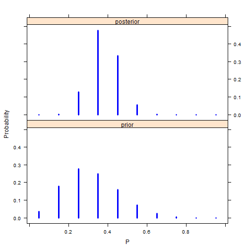

Here we can see a direct visual comparison between the prior and posterior probability distributions. Taking the evidence into account, we see that posterior probability peak shifts closer to .4. Overall, the main set of probability distributions is settled in-between .25 and .45 in terms of proportion (p).

2. Please replicate the sleeping habits analysis using a beta prior (in the session 1-2b).

Setting up the Beta Prior

The specification of a beta distribution is useful for bayesian analysis when it concerns the behavior of percentages and proportions.² The beta distribution is reflected by two shape parameters a and b, which can represent our prior beliefs about the proportion of students who get at least eight hours of sleep a night p. The code below creates the shape parameters for the beta prior by using the beta.select function, which utilizes our examples prior belief about two quantiles of p, the median (.3) and and 90th percentile (.5).³ Our example study believes that the median is equally likely (.5) to be smaller or larger than the median (.3), and that p is less than .5 (90th Percentile), with 90% confidence.

quantile1 = list (p = .5, x = .3)
quantile2 = list (p = .9, x = .5)

beta.select(quantile1, quantile2)

## [1] 3.26 7.19

The beta.select function provides us with the shape parameters of a(3.26) and b(7.19). This was done by first creating two variables that lists our beliefs about the median (.3) and 90th percentile (.5) quantiles, and using them as arguments in the beta.select function.

Evidence and Posterior

For the evidence and likelihood function, we retain the previous example study data of 11 college students out of 27 who receive at least eight hours of sleep. A conjugate analysis is possible with the beta prior, because once you combine the beta prior with the evidence, a beta posterior is computed. The code below sets up the beta posterior by using the dbeta command:

#set up the beta parameter values a and b from the beta.select output. n and y represent the study evidence values, with n taking on the number of observations, and y taking on the number of college students with at least eight hours of sleep.
a = 3.26
b = 7.19
n = 27
y = 11

#Visualize the beta prior and beta posterior by using the curve and dbeta functions.

curve(dbeta(x, a + y, b + n - y), from = 0, to = 1, xlab = "Proportion", ylab = "Density", lty = 1, lwd = 4)
curve(dbeta(x, a, b), add = TRUE, lty = 3, lwd= 4)
legend(.7, 4, c("Prior", "Posterior"), lty = c(3,1), lwd = c(3,3))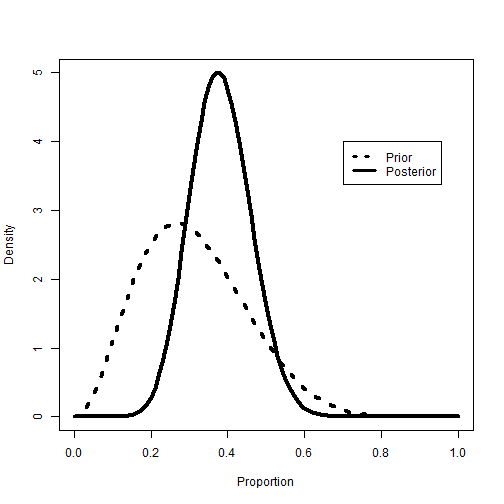

Here we can see a visualized comparison between the beta prior and posterior. As with the discrete posterior, the peak probability density for the beta posterior shifts towards .4 for p, after we take the study evidence into account.

Analyzing the beta posterior

This section looks at three different ways in which the beta posterior can be analyzed. For this, we ask the question; Is it likely that the proportion of heavy sleepers is greater than .5?

1) The first way to analyze this question is to compute the probability of p being greater than .5 by using the pbeta function, which is the beta distribution function. The code below calculates the probability of our question being right:

1-pbeta(0.5, a + y, b + n - y)

## [1] 0.0690226

The probability calculated is 6.9%, which is small. We can be confident that p is probably not more than .5, or more than half of college student sleepers.

2) The seoncd way to analyze this question is to create a credible interval estimate, which is a bayesian take on frequentist confidence intervals.⁴ Credible Intervals can be calculated by using the qbeta function in R. The code below calculates the credible intervals for the beta posterior:

#first create a vector in R for a 90% credible interval by using the 5th and 95th percentiles.
ninety = c(0.05, 0.95)

#qbeta function.
qbeta(ninety, a + y, b + n - y)

## [1] 0.2555267 0.5133608

The calculated 90% credible interval for our beta posterior is (0.256, 0.513). Again, it seems unlikely that p is greater than .5 because the credible interval only reaches past .5 on the uppertail, with the majority of the interval being below .5.

3) The third way to analyze this question is to use a simulation of a large number of values from the beta posterior. To do this, the rbeta function is used to generate a large amount of random proportion values based on the beta shape paramters. The code below computes the simulation and visualizes the results using the hist function:

#Set a seed before simulation, this allows others to replicate the code and find the same values.
set.seed(1234)

#Now perform the simulation and visualization.
sim <- rbeta(1000, a + y, b + n - y)
hist(sim, xlab = "p", main="")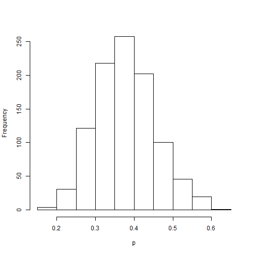

The histogram above shows newly simulated sample for p. Next we can replicate the previous two posterior analyzes by using the sum and quantile functions. The code below calculates the probability and credible interval for the question of interest:

#estimate the probability of p > .5:
sum(sim >= 0.5)/ 1000

## [1] 0.067

#estimate the 90% credible interval for the 5th and 95th percentiles:
quantile(sim, c(0.05, 0.95))

##        5%       95% 
## 0.2627529 0.5196811

Both the probability (6.9% vis a vis 6.7%) and the credible interval estimates (0.25, 0.51 vis a vis .26, .52) are very close to the original exact values of the beta posterior. The results still lead to the analyst to conclude that p is unlikely to be greater than .5, but what if we can increase percision by greater simulation? The next block of code replicates the previous simulation procedure but with 1,000,000 generated values for p instead.

#Simulation with 1,000,000 values of p.
sim2 <- rbeta(1000000, a + y, b + n - y)

#Estimate probability and credible interval.
sum(sim2 >= 0.5)/ 1000000

## [1] 0.068864

quantile(sim2, c(0.05, 0.95))

##        5%       95% 
## 0.2553036 0.5131889

After increasing the simulation to a 1,000,000 values of p, we find even closer estimates of the probability of p > .5 (6.9% vis a vis 6.8%) and the credible interval (0.25, 0.51 vis a vis .25, 0.51). We can be fairly confident in our previous findings concerning the question. After taking into account the study evidence, it is unlikely that the proportion of college students who have at least eight hours of sleep a night is greater than .5.

3. Please replicate the birth rate comparison analysis using a Poisson Likelihood (in the session 1-5).

For the study of birth rates amongst women with, and without college degrees, we utilize the Poisson model. Birthrates qualify as count data, which can be better analyzed by using poisson and negative binomial modeling.

Setting up the Prior

For a Poisson likelihood model, one can use a gamma conjugate prior. Again, this type of prior only needs to model our beliefs about two parameters, a(occurances) and b(intervals). The code below sets up our gamma prior.

a = 2
b = 1

Evidence and Posterior

Next, we wish to take into account the evidence about birthrates amongst women without college degrees, and with college degrees. This data comes from the General Social Survey (GSS), which interviewed women on educational attainment and number of children. From here, group 1 defines women without a college degree, and group 2 defines women with a college degree. The code below establishes the evidence (data) for both groups of women, and then finds the 95% credible interval for number of children for each group.

#data for group 1 (women without degrees)
n1 = 111 #number of women without degrees
sy1 = 217 #number of successful trials (i.e. children born)


#group 1 posterior mean
(a + sy1) / (b + n1)

## [1] 1.955357

#group 1 posterior mode
(a + sy1-1) / (b + n1)

## [1] 1.946429

#group 1 95% credible interval

qgamma( c(.025, .975), a + sy1, b + n1)

## [1] 1.704943 2.222679

The posterior mean number of children born to group 1 is 1.95, the mode is 1.94, and the 95% credible interval is (1.70, 2.22). The code below computes the posterior data for group 2.

#data for group 2 (women with degrees)
n2 = 44 #number of women with degrees
sy2 = 66 #number of successful trials (i.e. children born)

#group 2 posterior mean
(a + sy2) / (b + n2)

## [1] 1.511111

#group 2 posterior mode
(a + sy2 - 1) / (b + n2)

## [1] 1.488889

#group 2 95% credible interval
qgamma(c(0.25, .975), a + sy2, b + n2)

## [1] 1.383810 1.890836

The posterior mean number of children born to group 2 is 1.51, the mode is 1.48, and the 95% credible interval is (1.17, 1.89).

Posterior Group Comparison

Comparing the posterior results between group 1 (without degrees) and group 2 (with degrees) shows that women with degrees appear to have less children (y) on average than their counterparts without degrees (1.51 versus 1.95). The posterior credible intervals also show two mostly different ranges for number of children (y) had by both groups of women (1.70, 2.22 versus 1.17, 1.89). The code below creates a visualized comparison of the gamma prior, posterior for group 1, and posterior for group 2:

curve(dgamma(x, a + sy1, b + n1), from = 0, to = 5, xlab = "y", ylab = "Density", lty = 1, lwd = 3)
curve(dgamma(x, a + sy2, b + n2), from = 0, to = 5, add = TRUE, lty = 1, lwd = 1)
curve(dgamma(x, a, b), from = 0, to = 5, add = TRUE, lty = 2, lwd = 2)
legend(3, 2, c("Posterior without degrees", "Posterior with degrees", "Prior"), lty = c(1, 1, 2), lwd = c(3,1,2))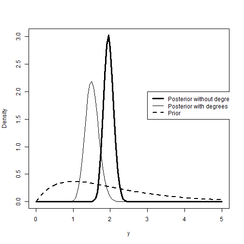

The plot above confirms the previous observation about the posterior comparison between the two groups of women. Women without degrees peaks around 2 children, while women with degrees peaks at around 1.5 children.

Birth Rate Prediction

To make predictions about the number of children women will have depending on their college degree status, we can utilize the posteriors found above with a negative binomial distribution. This can be done in r by using the dnbinom function. The code below creates predictions of birth rates (y) for both groups of women:

#quantile range for predicted number of births
y = 0:10

#predicted birth rate for women without degrees
predict1 = dnbinom(y, size = (a + sy1), mu = (a + sy1) / (b + n1))


#predicted birth rate for women with degrees
predict2 = dnbinom(y, size = (a + sy2), mu = (a + sy2) / (b + n2))

The code above creates predicted probabilities for number of children born on an interval of 0 to 10. The dnbinom function uses two arguments to create the predicted probabilities. The first is the size, or dispersion paramters, and the second argument is the mean.

The code below creates a visualized comparison of the predicted probabilities for both groups of women:

plot (y, predict2, type="h", lty=1, lwd=5, col=rgb(0,0,0,1/5), 
      ylab="Predicted" ) 
lines (y, predict1, type="h", lty=1, lwd=4, col=rgb(0,0,0,1/2))  
legend(5,0.2,c("Predicted w/o degrees","Predicted with 
degrees"),lty=c(1,1),lwd=c(4,5), col=c(rgb(0,0,0,1/2),rgb(0,0,0,1/5)))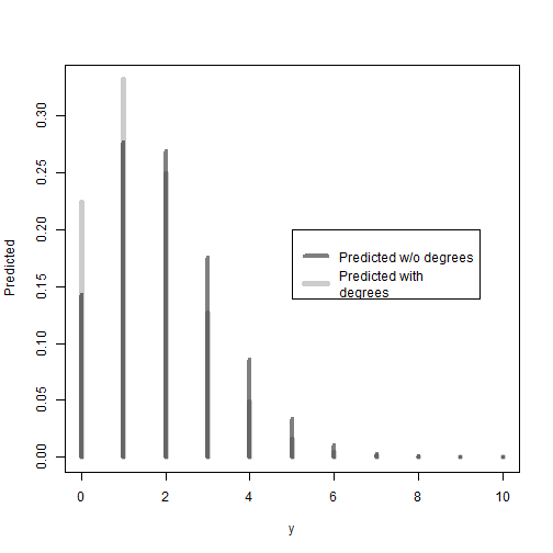

As expected, the plot above shows that women without degrees have higher predicted probabilities to have two or more children. In turn, women with a degree have relatively higher predicted probabilities for having a single child or no child, when compared to women without a degree.